How I Measured The Height Of Clouds By Looking Out The Window

As I'm sitting down to write this, I realize that the last time I posted anything to this blog was December of 2015!  This was just after a series of deadly tornadoes ripped through North Texas the day after Christmas.  Since that time, I've learned a lot more about the weather have gone on a number of successful (and some not-so-successful) storm chases.  I started a small Facebook weather page too (innocently plugged here) to not only give people more info about weather for North Texas (sometimes Chicagoland and West Michigan too) but as another outlet for posting my weather photos.  Sure, posting pictures is fun and I'm going to continue to do that of course, but I still think that writing one's thoughts down after an experience like chasing or experiencing cool weather can really help to convey the emotions of what it was like to be there.  And of course, it can help others to learn and hopefully find the same excitement as me.   With that, here's to [hopefully] more posts!

I'll preface this article by saying that it's going to be SUPER NERDY.  I'm totally fine with that.  I've always been nerdy and I'm sure I always will be.  Oh..yeah - there's going to be some math (or "maths" as the British say) - but not too much I promise.  OK here goes:

I work for an architecture firm located in the West End of downtown Dallas.  We are currently constructing an expansion to our existing building.  It's fascinating to watch the progress to say the least.  As I was taking a short break from work this afternoon, I found myself looking out the window from my desk watching the flurry of construction activity below.  I quickly noticed something which instantly drew my attention away - clouds!  It's not like clouds are anything new, BUT we've been under a fairly dry weather pattern lately - so much so that clouds have been few and far between.  Some folks love that kind of weather.  Call me crazy, but I'm the opposite.  Give me clouds!  Give me storms!  Anytime I can look outside and see clouds, I'm happy.  But I wasn't expecting to see clouds today, except maybe a few cirrus here and there.  At this point you're thinking - wow! - those must be some cool clouds.  Well, no.  They weren't cool  There were just there.  I'm sure they were unnoticed by 99.9% of everyone else.  But they were there nonetheless!  And I saw them.  Here's was my view.  See them - waaayyy off in the distance....

Told you it was boring!  But it got me thinking - I wonder if I can see these on satellite?  You see, since my last post, a new weather satellite called GOES-16 has gone into operation.  This satellite is AWESOME - providing very high-resolution images in a much faster time than the previous generation of weather satellites.  It also can take 1-minute increment snapshots, giving a whole new way to experience cloud animations.  It's an amazing tool to say the least.  Pulling up the view for North Texas yielded this.

To the untrained eye, this may not look like much.  Here's an annotated version.

As you can see from my vantage point (near "DFW"), the clouds I saw were nearly to the Red River!!  This really surprised me.  I didn't think they would be that far north.  Naturally, that led me to my next question - how far away are they?  As you can see from the satellite picture, lakes around the DFW region show up dark - which means they can be very easily identified by their shape.  Assuming the clouds I photographed earlier were the same ones I circled above in yellow, then I determined that they were a bit further north of Lake Ray Roberts.  Thanks to Google Maps, it made measuring the distance pretty easy.

Based on the satellite view and Google Maps,  I estimated that the clouds in the picture were approximately 54 miles away.  But that's just in one direction.  I wondered if there was a way to calculate their heights?  This is where the math (and a little imagination) comes in!   Imagine if you will, 3 points in space - me (the observer), a point roughly 54 miles distant, and directly above that a point representing the clouds.  In essence what I've just described is a RIGHT TRIANGLE.  BINGO!  Can't see it?  Check this out....

In this view, my unknown value "X" is the height of the clouds.  This is what I need to solve for.  Given the 3 points I mentioned earlier, we can use trigonometry (more specifically the TANGENT operation) to estimate what the heights would be.  However I would still need to estimate one other piece of the equation - the angle of the clouds above the horizon - as seen from my perspective.  After looking up some crude ways of measuring degrees using my hands (I must have looked like a real tool holding out my hands toward the window!!!) I came up with my guess of 7 degrees.  I now had all I need to work out the problem.  Here's what I jotted down.

6.63 miles. This was my guess.  Was I right?  Beats me!!  I had no real way of knowing.  But like I was taught in school - go back to make sure your answer makes sense.  Ok.  Sure.  Um..how?   Oh yeah - SOUNDINGS!

I won't get into the nitty gritty of soundings here (I've written about them in previous posts) but I will briefly say that soundings are a tool which give a good idea of the vertical make up of the atmosphere by using a weather balloon to measure data like temperature, dewpoint, winds, etc. 

A few clicks later yielded this...

Remember that the bigger distance between the red (temperature) and green (dew point) lines, the drier the atmosphere is at that given point.  The above sounding indicates very dry air in place - much too dry to support clouds.  

BUT

Look here...

This is the area on the entire sounding where the 2 lines are closest - just above the 9 KM line and is the area where clouds would be most likely to be.  I switched over to the raw data view to see the numerical values which form the basis of these lines.  I was looking for the line which contained the smallest separation between the temperature and dewpoint - something called the dewpoint depression.

And there it is - 286 mb - or 9770 meters above the ground.  But how does that tie into my guess of 6.63 miles?  For that, it's just a matter of conversion:

My guess of the height of clouds:  6.63 miles = 10669.95 meters

Sounds data indicating likely area of clouds = 9770 meters

Difference?   900 meters.  Just under 1 KM!   WOW!  Not a bad guess overall for just looking out the window.  

-Andrew

Possible Severe Weather for North Texas on the Eve of Halloween?

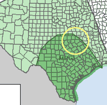
I'm going to preface this post by saying that I'm NOT a weather forecaster, nor do I pretend to be one.  However, in my self-study of weather, I've noticed certain ingredients that when added together in just the right amounts can make for some unsettled weather.  The problem is of course is that the weather is ALWAYS changing and what looks good today, may not look good when the time comes.  Here's what I'm mean.  Confidence is increasing that Friday, October 30, 2015 will be another rainy day for North Texas.  However, there is a chance, albeit low at this time, for severe weather.  This is the SPC Outlook for Day 3 - Friday, October 30, 2015.  Already, some parts of north Texas are shown in the MARGINAL RISK area.

The enlarged view shows a good portion of the DFW Metroplex under the MARGINAL RISK area including Tarrant, Johnson, Ellis, and parts of Dallas county.

Severe weather requires 4 key ingredients:  moisture, lift, instability, and wind shear.

Let's look at the ingredients in more detail:
NOTE:  All images are taken from the GFS weather model, 06Z initialization on 10/28/15 @ 21Z (4 PM)

MOISTURE
In order for it to rain, you need moisture!  For that we can look at the forecast dew points.

This image shows forecast dew points for North Texas in the low to mid-60s - which is plenty of moisture in the atmosphere for severe weather.


LIFT
The jet stream is a fast-moving "river" of air in the upper atmosphere which impacts our weather.  The shapes the jet stream can take are a result of high and low pressure areas.  A trough is a large U-shaped structure in the jet stream which indicates a low pressure area - generally responsible for poor weather.  When wind approaches a low pressure center, it tends to slow down around around the center region, then quickly speed up and eject out of it.  This image is taken from the GFS weather model and shows the predicted winds at 500 mb (millibars - a measure of pressure) or about 18,000 feet up.

The U shape is clearly visible west of Texas and the winds ejecting from it are sailing directly over us.  This creates lift in the atmosphere by a process known as upper level divergence.  An oversimplified example of this is a line of cars accelerating at a green light.  As the cars begin to speed up, the distances between them gets larger.  In the atmosphere, when the wind "diverges" high up, winds from below are lifted up to fill those "gaps".  Lift helps to raise air up so it'll cool, condense, and rain.


INSTABILITY
Instability is a measure of the tendency of air to be lifted.  This is highly dependent on temperature and moisture.  If the temperatures above us don't cool down in fast enough going up in to the atmosphere, this impedes surface air from wanting to rise.  In this case, we say the air is stable.  If air is unstable (a higher instability number), air will have a tendency to rise.  This chart shows a forecast sounding (a vertical temperature and moisture profile) for central Hill County on Friday at 4PM.

Note the blue line.  See how it doesn't go very far to the right of the red line, if at all?  At a very basic level, this means that there will not be a large amount of instability in the atmosphere.  This factor alone is a large reason why the severe weather chances are low.  If that blue line were much further to the right - creating a large space between itself and the red line, severe weather chances would most certainly increase.  But again, this is a forecast weather model and not a direct measurement (it's in the future keep in mind), so things are of course subject to change.


WIND SHEAR
Wind shear is a change in wind speed (speed shear) or direction (directional shear) with height.  In other words, winds at the surface tend to change direction and/or speed the higher you go in to the atmosphere.  It's not uncommon to have winds coming out of the south or southeast at ground level and winds coming from the west at 500 mb (18,000 ft).  Wind shear plays a large role in the longevity and strength of severe storms.

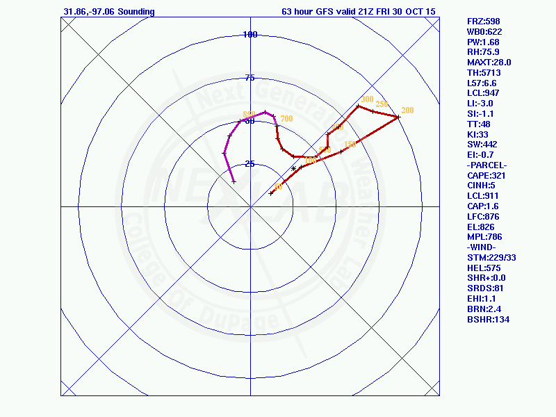
To get a good look at wind shear, we can use a something called a hodograph which plots wind speeds in a certain way on a circular graph.  The shape of these wind speeds can give a good indication of the type severe storm and even if the possibility of tornadoes exists.

Without getting into all the nuts and bolts, the key thing about this image is the large circular shape in purple.  This is the graph of the forecast lower level winds.  The strength and shape of this curve indicates that at this time, (assuming that all other ingredients come in to play) that tornadoes are possible.  Keep in mind that A LOT has to go right for tornadoes to develop - much the same way that in addition to flour, lots of ingredients have to come into play to make a cake.

As I mentioned before, this is just one slice on information from one specific weather model and is NOT meant the be an authoritative forecast.  In fact, this is probably wishful thinking on my part and are a result of me wanting to chance some storms!  While the wind shear, lift, and moisture look promising, the lack of instability may turn this whole event sour.  Regardless, let's see how these ingredients shape up and keep an eye to my Faceook page for more up-to-date info!

-Andrew

Bastrop County Wildfire Smoke Demonstrates Temperature Inversion

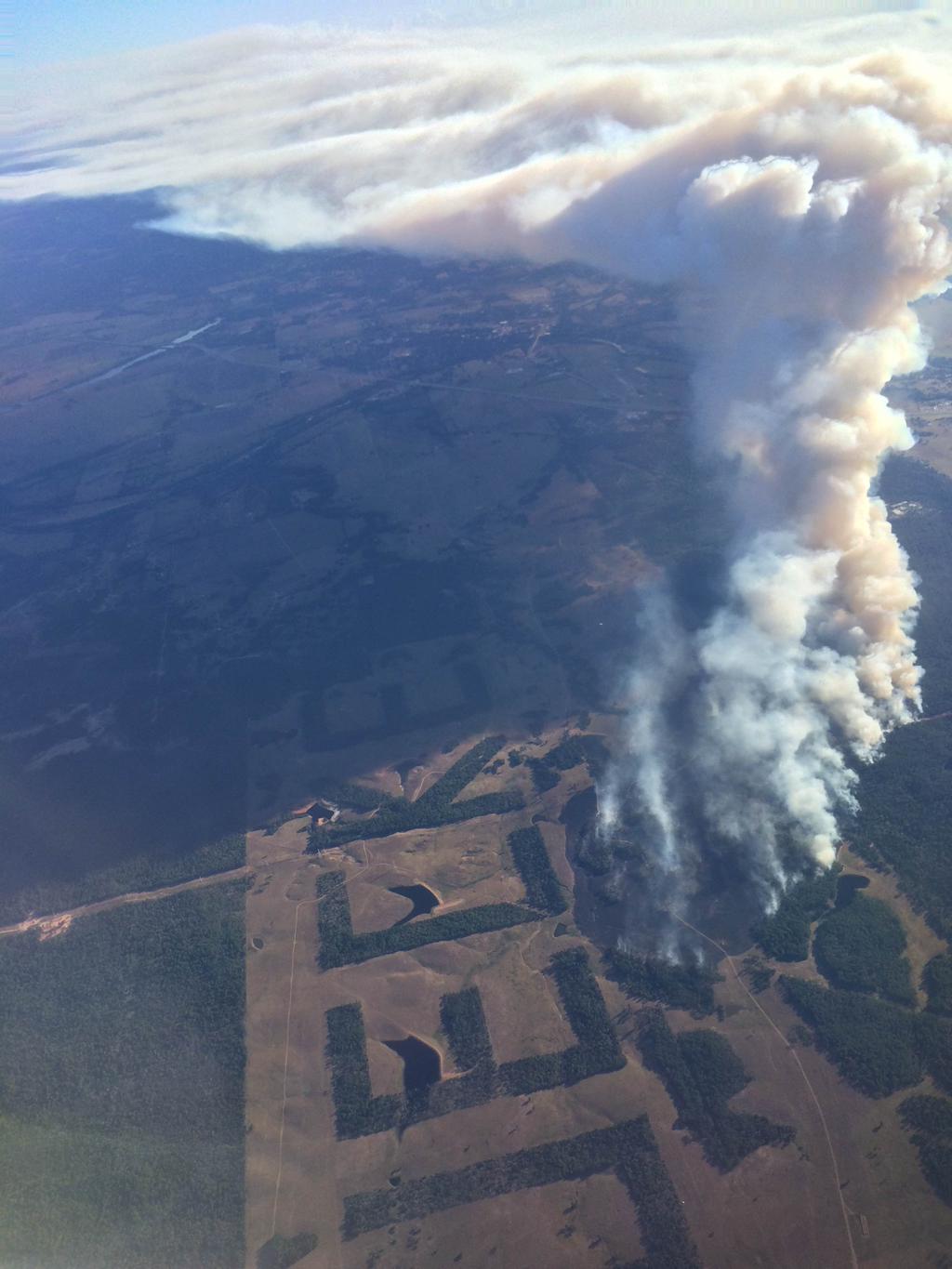
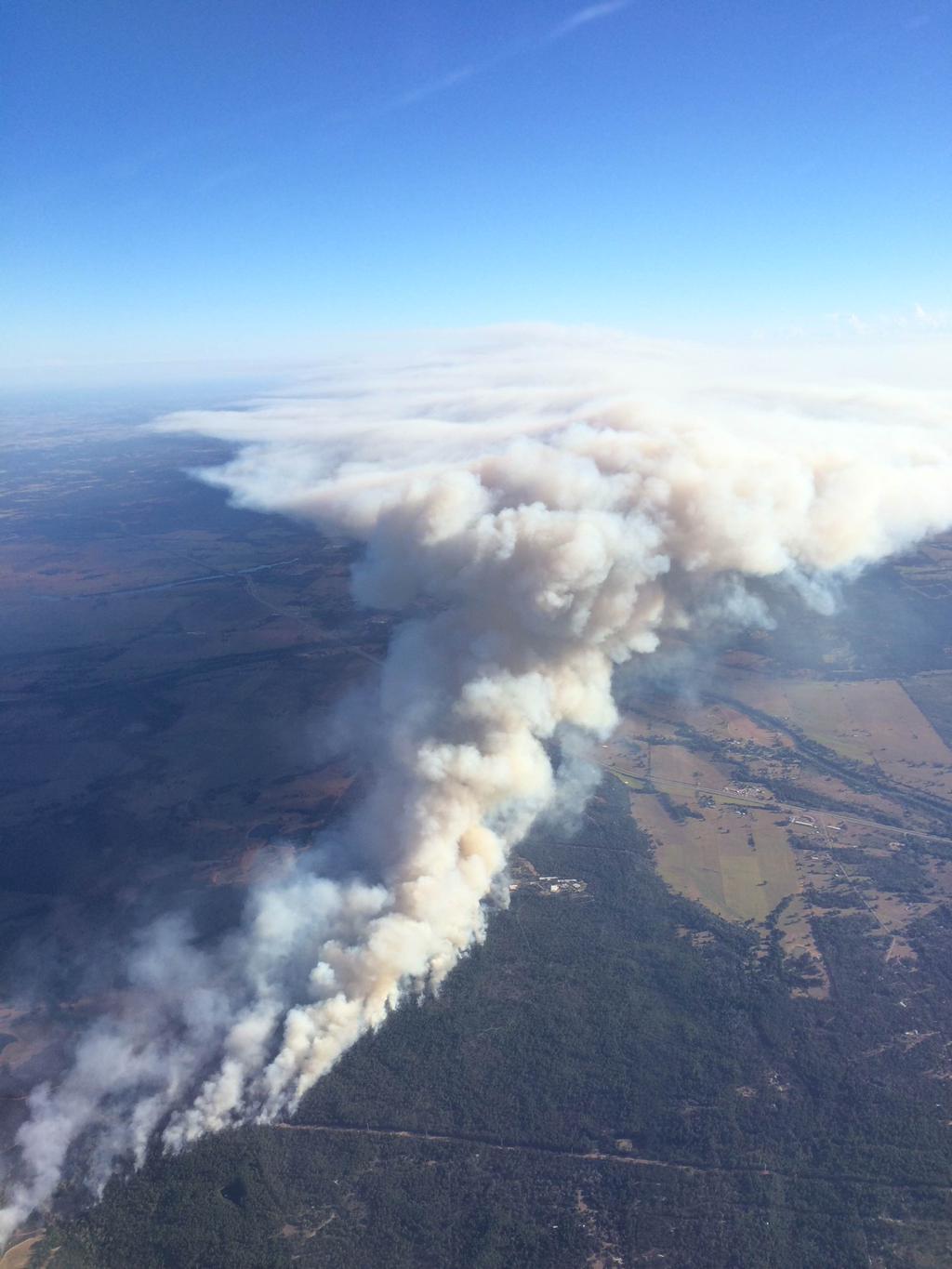
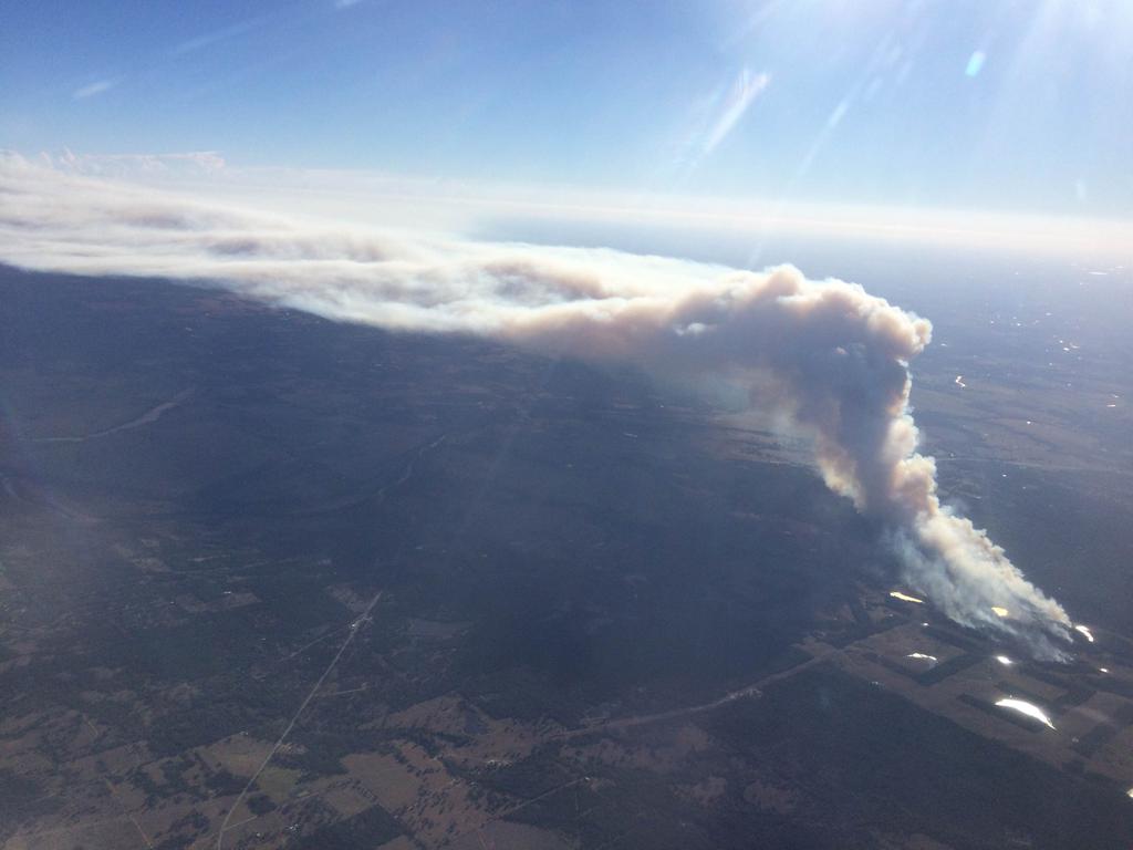
Bastrop County, Texas (about 190 miles south of DFW) is yet again dealing with severe wildfires.  Back in 2011, that same area suffered through what became the most destructive series of wildfires in Texas history.  Luckily the current blaze is nowhere near that size.  What spurred me into writing this post, however, wasn't the fire itself but the smoke from the fire.  The following pictures were snapped by an airline passenger who happened to be flying in the vicinity of the fire.  This person proceeded to tweet them to an Austin-area TV station and from there they made it around the Twitterverse.

(pictures credited to an unknown Twitter user)

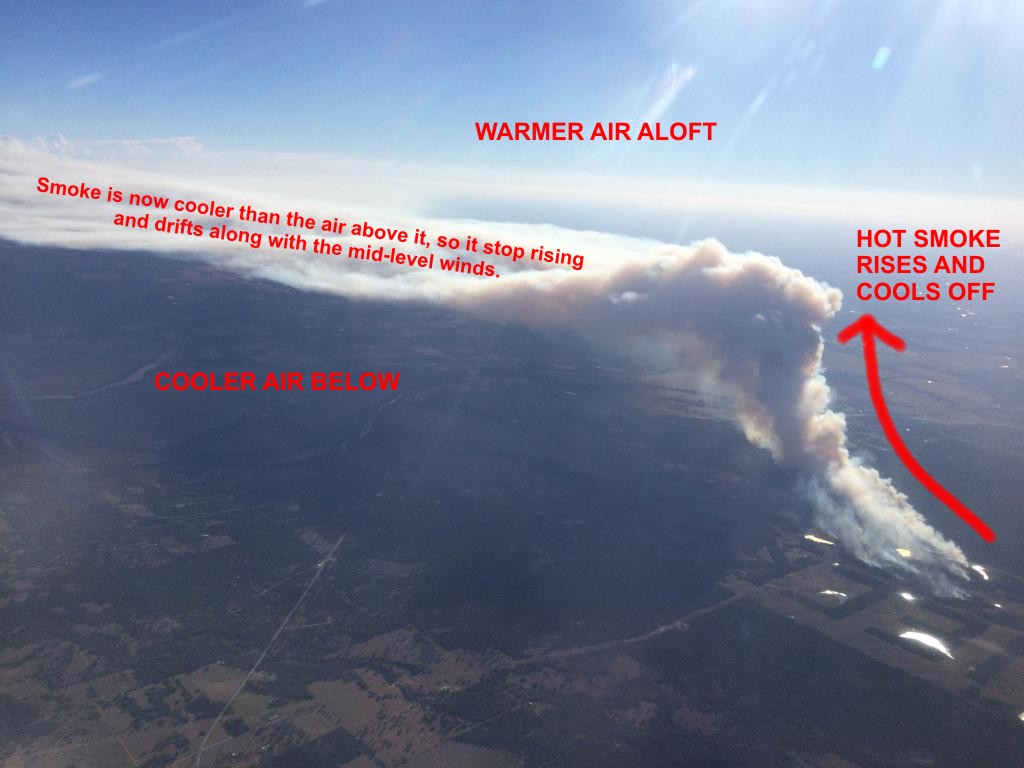
Look at the 3rd picture in particular.  Notice how the smoke seems to stop rising and instead gets carried downstream by the mid-level winds?  It's almost like that smoke hit a ceiling and couldn't get any higher.  In effect, it did!  This is a perfect illustration of a temperature inversion.  Temperature inversions are not uncommon and are the cause of thunderstorm anvils and in some cases fog!

You see, when a chunk of air (the technical term is parcel) is warmer than the air around it, it's considered to be buoyant and so it rises.  Smoke from wildfires is hot - much hotter than the environmental temperature - so up into the air it goes.  The smoke will continue to rise until it hits a level in the atmosphere which is the same temperature or warmer than itself.  At this point, the smoky air is no longer buoyant so it stops rising.  Incidentally, This is the same reason why cumulus clouds only grow so tall - because the updrafts which created them cool down and become the same temperature as their environment.

Here's an annotated version of the Bastrop County wildfire.

But why is this called an "inversion"?  To illustrate this, let's break out the old Skew-T chart.  I've referenced this before many times.  A Skew-T is a meteorological chart used for viewing the vertical temperature profile from ground level to upper atmosphere; a cross-section of the atmosphere in essence.  Under normal conditions, the air at the surface is warm (relatively speaking) and will cool off the higher you go into the atmosphere.  Graphed on a Skew-T diagram a standard temperature plot would look like this.

See the red line?  This is the vertical graph of air temperatures.  This chart was from the DFW area on 10/13/2015 at around 7 PM.  The line generally runs from right to left the higher up you go.  The temperature lines are "skewed" to the right, hence the name Skew-T (Temperatures are in Celsius, notated at the bottom of the chart).  Let's now compare that image to this.

This is from 10/14/2015 at 7 AM - about 12 hours after the previous example.  Notice how the bottom of the red line starts to go to the right and then curves back around?  This demonstrates that the layer of air near the surface actually gets warmer with height!  This is the temperature inversion! In this particular example, the air near the surface cooled down significantly overnight (22 degrees from the previous evening), yet the air aloft remained warm.  As an aside, if the air near the surface had more moisture, it would be this same type of atmospheric setup responsible for fog.

-Andrew


P.S. Anyone notice the letters on the ground in the first picture of the wildfire?  More info here!


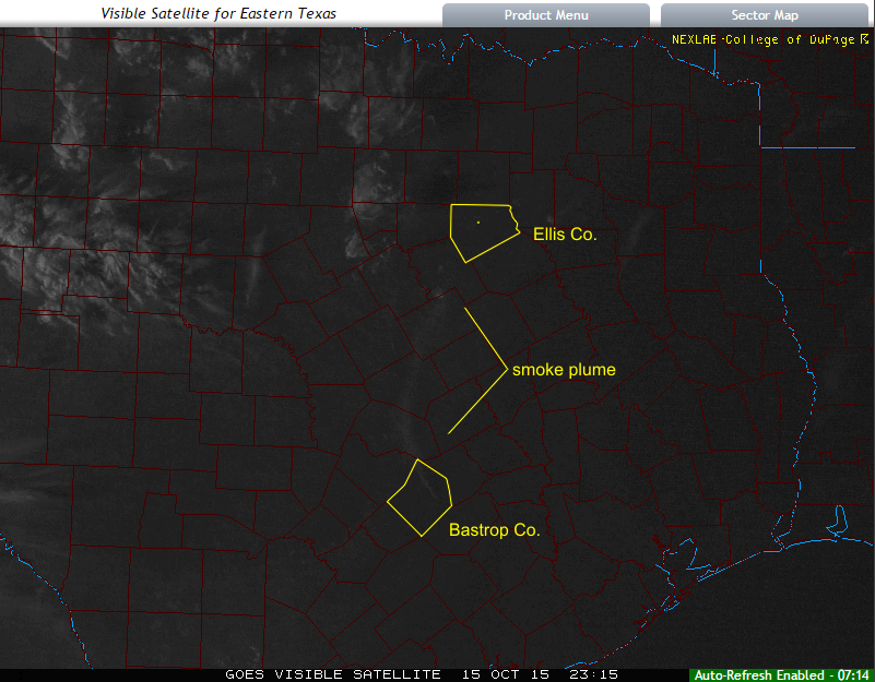
UPDATE: The smoke plume from the fire was visible on satellite today.

10/15/2015 Update:  Taking the kids to the bus stop this morning, I was hit with the distinct smell of smoke - almost like somebody had a fire going.  The smoke from the Bastrop county wildfire had made it as far as the DFW area.  Looking at the visible satellite imagery from this evening, here's why:

The smoke plume was drifting directly towards us!  I wouldn't be surprised if I woke up to another smoky morning....

When Something In The Sky Seems Odd

File this post under miscellaneous drivel.

I am a very habitual person.  When I get into a routine, it's hard for me to break it.  Ever since getting into meteorology, I've gotten into the habit of checking the morning and evening soundings for the DFW and surrounding areas.  Soundings can show a great deal about the vertical makeup of the atmosphere.  Here are the morning soundings for today - February 9, 2015.

 

 

 

As the pictures indicate by the wide spacing between the red (temperature) and green (dew point) lines, the air in the DFW region is very dry - much too dry for clouds to form.  However, when I picked up my oldest daughter from theater practice tonight, I noticed this to my north.

 

 

The whole time I was looking at this, I kept thinking to myself, "This shouldn't be there.  What's going on?"  I also couldn't get over that distinctive arrowhead shape.

 

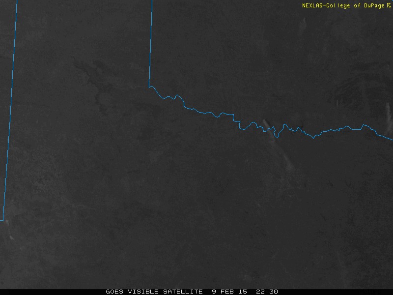
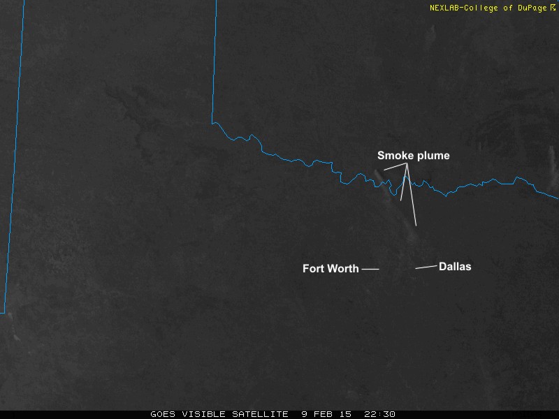
When I arrived home, I pulled up the 1KM visible satellite feed and got the answer to my question.  The "cloud" wasn't really a cloud at all, rather a smoke plume from southern Oklahoma - originating some 115 miles away!

 

This was the visible satellite image from 2230Z (5:30 PM CST)

 

 

The squiggly blue line running west to east is the Red River, which is the border between Texas and Oklahoma.  About midway though the Red River is a white/gray plume of smoke running from the northwest and blowing southeast.  Here's another view to give you an idea of scale.

 

 

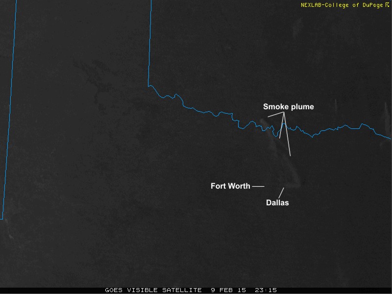
The image from 45 minutes later - (2315Z, or 6:15 PM CST), showed from above exactly what I had snapped from ground level. 

 

 

Easily visible in this image is that same arrowhead shape that I had seen from below.  When running the animation loop of the visible satellite feed, I noticed that this wasn't the only fire in Oklahoma today - but this was certainly the most prominent.  In other parts of the state, I read that the forest service were doing controlled burns in some of their forest preserves.  There didn't look to be a forest preserve near the origin of this fire so I'm not entirely sure of the cause.  So, while not earth shattering, I thought it was kind of cool to correlate a photo taken on the ground with an image from a satellite orbiting roughly 22,000 miles above the ground!!



 

Can't We Get Rid of This Persistently Nice Weather?

Am I going crazy?  Why would anyone want to get rid of such nice weather?  Surely I must be joking, right?  Well, yes and no.  While I do enjoy nice sunny days, I very much long this time of year for the excitement of the spring storm season.  The clean, dry air of high pressure days, while pretty, just doesn't do it for someone who always is looking at the clouds.  A quick view of our extended forecast for North Texas puts daytime highs in the 60s and 70s - with only a few days mixed in with very low precipitation chances.  Boo!  (Can you feel the sarcasm dripping from this post??)

As it turns out, I actually can blame this weather on something:  a Rex Block

Who is Rex Block?  Well, a Rex Block isn't a who, but a what.  This is a meteorological term for a specific type of blocking pattern.  Blocking patterns are relatively stationary weather patterns that block other systems from coming through.  The Rex Block is a special type of blocking pattern in which an upper level center of low pressure is situated directly southward of an upper level high pressure center.  It was named after Dr. Daniel F. Rex who named this pattern in 1950.  Here is an idealized diagram:

Winds from the west encounter the high pressure area and begin to flow clockwise around it, then start to flow counter-clockwise around the low pressure area.  In other words, the winds blow in a backwards S pattern from north to south.  As there little west-east flow, this pattern can persist for days.

Here's what our current weather pattern looks like.  This image is taken from the NAM weather model.  It shows the 500mb weather patterns (winds at around 18,000 ft. above the ground).

 

There's a few features that I need to point out so that all of this makes some sense.  I've added a large, blue H over northern Mexico.  This (as I'm sure you've seen countless times on other weather maps) is an area of high pressure.  High pressure generally gives clear skies and dry air - exactly what we have today. Also, take a look at the solid black lines.  See how they make patterns that look like a large right-side up and upside down U?  Now look at how Texas is west of one of these U-shaped features.  Generally speaking, the western side of the U tends to have sinking air (i.e. high pressure) and fair skies, while the eastern side of these U shapes generally have rising air (low pressure) and cloudy skies.  

 

The large, red L is of course a low pressure area - responsible for clouds and rain - exactly what is happening in Washington and Oregon today.

 

As the NAM continues over its 84-hour forecast period, it shows the low swooping down from the Pacific Northwest, but then starts to retrograde (or move westward) and finally positions itself on the north end of the Baja Peninsula, directly southward of another high pressure ridge.  This pattern now forms the classic Rex Block.  Here's the 84-hour forecast NAM view.

 

 

You'll notice how Texas continues to be generally westward of one of those U shapes.  Again, this region generally has sinking air and fair skies.  When you add the effects of the Rex Block, it's going to ensure that we have clear sailing for a long time to come.  The GFS weather model also shows a Rex Block for the same time period (roughly 84-hours out).  However, because the GFS forecasts out to 240 hours, it also shows that we could be in for a nice change (and by that I mean RAIN) by early next week. 

 

Until then - enjoy the weather!

 

 

Altocumulus Castellanus Clouds - The Jellyfish of the Sky

One of the neat things about studying meteorology (and weather in general) is that sometimes you come across something very cool that most people would take for granted.  In my reading about different weather phenomenon a few weeks back, I ran across an article on something called Jellyfish Clouds.  These clouds are fairly rare and form when a layer of moist air rises upwards due to convection and becomes sandwiched between two layers of drier air.  Sometimes when these clouds form, they drop precipitation into the lower dry layer and it begins to evaporate.  The result is a cloud leaving a wispy tail below it which resembles it's namesake - a jellyfish!

On Friday, September 26, 2014, the drive home from work was pretty commonplace and uneventful.  A few miles away from home, I noticed some interesting clouds to my south (yes, I spend a lot of time looking UP at the sky when I probably should be looking at the road!).  Be that as it may, I finished my drive home and when I got into the driveway, I immediately shut off the car and snapped this picture:

 

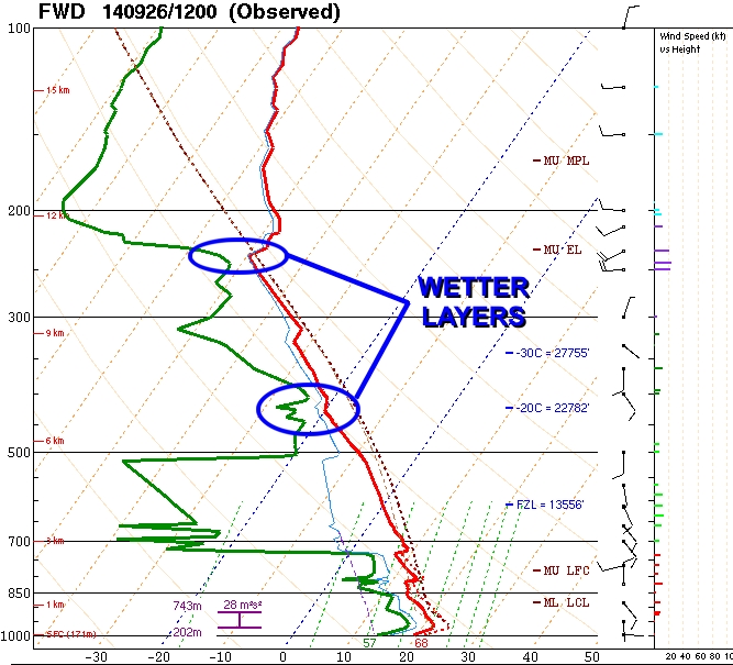
 I was pretty excited as these looked very much like the jellyfish clouds I had read about a few weeks prior.  However, I didn't want to make too much of it, so I decided to check the sounding data for that day to confirm my suspicions.  I've referred quite a bit to soundings in my previous posts, and it's a topic about which I solely need to devote a topic, but to briefly recap a sounding can be thought of as a cross section of the atmosphere from the ground level all the way up through the troposphere (the area of the atmosphere where all the weather takes place).  Soundings come out at 8AM and 8AM during daylight saving time (7AM and 7PM otherwise).  Data is generated by an instrument called a radiosonde which is attached to a weather balloon.  This instrument and balloon are released from National Weather Service offices all around the country and help meteorologists get an idea of the makeup of the atmosphere above.  They measure temperature, dew point, wind speed and direction.  It was about 6 PM when I arrived home, so the only thing I had at my disposal were the morning sounding.  Here's what it showed:

This graphic contains a TON of information, but the focus for the rest of this article will be on the upper left corner.  This plot - showing the red and green lines - is a graphical depiction of both the temperature (red line) and dew point (green line) starting at the surface (the bottom of the graphic) rising up to some 15-17 km (49,000 - 55,000 ft.) in the air.

 

The first thing you notice is that the red and green lines are fairly close together near the bottom.  The lowest layer - often referred to as the PBL, or Planetary Boundary Layer, shows that due to the proximity of the lines, there is a fair amount of humidity in the air.  Above the PBL, the green line veers sharply to the left.  This indicates that the next layer up is very dry.  Above that, it gets more humid, then dry again, then humid, then dry.  Who knew so much was going on above our heads!!  Here's a better explanation:

 

 

 

In these dry layers, no clouds can form as there is simply not enough moisture.  However, when the lines get close, this indicates that there is sufficient humidity for clouds to form.  In fact, depending on where the layers are, you get different types of clouds!

 

 

 

Remember above when I said that jellyfish (altocumulus) clouds form in a moist layer which is sandwiched between two drier layers?  Well, this is exactly what we had in the atmosphere that day.  In other words, this did confirm to me that, yes, what I had captured earlier were the elusive jellyfish clouds!  From the morning sounding it looks like they were forming above the 6 km (~19,000 ft) mark.  The precipitation which was dropping from them fell into a very dry layer below 6 km.  This was the cause of the wisps beneath the clouds.

 

When the evening soundings were posted, I checked those one last time to see if the data would still support my findings.  Sure enough, although it was quickly drying out, the comparatively humid layer above 6 km was still present.  As I write this article, I'm still jazzed that I was able to capture a fairly rare phenomenon.  Can't wait until the next occurrence!!

 



 

BUT WAIT!  For those of you who haven't dozed off yet, you may have noticed that altocumulus clouds formed in a region where the air temperature is -20 C (-4 F).  How is this possible to have liquid water exist at a temperature below freezing??  Well, believe it or not, this is a process called supercooling and involves a whole branch of could physics (yes, there is such a thing).  This, however, would require it's own article......

 

-Andrew

 

 

 

 

The Dangers of Downbursts from Pulse Severe Thunderstorms

On Saturday, August 16, 2014, the Storm Prediction Center put all of North Texas into it's lowest probability category for severe weather. 

Our area didn't even make it into a SEE TEXT region, yet with our moderately unstable air and weak wind shear environment, conditions were favorable for pulse thunderstorms which were capable of producing a phenomenon called DOWNBURSTS.

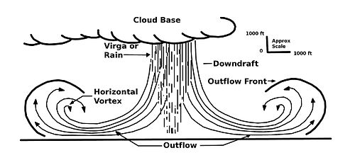
A pulse thunderstorm is a single-cell thunderstorm forms and dissipates relatively quickly and typically doesn't yield any severe weather.  However, some pulse storms grow fast enough and drop enough rain to produce a downburst.  A downburst occurs when rain-cooled air falling out of a thunderstorm hits the ground and begins to spread out in all directions.  This expansion of winds (called outflow winds) can sometimes reach 100 MPH and cause quite a bit of damage!  The easiest way to visualize this is to imagine pouring water out of a glass and onto the ground.  As the water slams into the ground, it immediately fans out in all directions, pushing air in front of it.  Is this forward motion that can drive winds as far as 50 miles away from the original storm.  Here is a good visual representation, shown in cross-section. (h/t Wikipedia)

There are actually 2 varieties of downbursts - wet and dry.  A wet downburst happens when rain falling out of the thunderstorm reaches the ground.  A dry downburst happens when rain falling from a storm evaporates before hitting the ground.  In either case, it's the outward-spreading winds from this cooler, sinking air that is responsible for causing damage.  Downbursts smaller than 2.5 miles in diameter are called micro downbursts or microbursts.  Downbursts greater than 2.5 miles in diameter are called macro downbursts or macrobursts.

Let's examine a real-world example of downbursts.  This example begins northwest of Fort Worth, TX.  At 3:02 PM, the National Weather Service issued a severe thunderstorm warning for northwest Tarrant and northeast Parker county.

 

Although the radar returns look unimpressive, there were some interesting things that were about to happen.  One of the dangers with downbursts and the storms associated with them is the speed in which they form, drop their rain-cooled air, and eventually collapse.  The following 5 snapshots of radar reflectivity and radar velocity start at 3:12 PM (about 10 minutes after the initial warning was issued) and ends at 3:31 PM - a span of only 19 minutes!! 

 

TIME 3:12 PM

The first thunderstorm core is in the process of growing. 

 

 

 

TIME 3:17 PM

The first thunderstorm core is still in the process of growing, while a new core is forming to the northwest.

 

TIME 3:22 PM

The first thunderstorm core has matured fully and has begun to produce a downburst (visible on the right side of the image).  The velocity view clearly shows that winds directly underneath the thunderstorm are hitting the ground and are spreading out.  The red colors indicate winds that are blowing away from the radar, while the green colors show winds blowing toward the radar.  The second thunderstorm core continues to grow.

 

 

 

TIME 3:27 PM

The first thunderstorm core is now in the dissipating (or dying) stage.  Reflectivity values (intensity of rain) has dramatically dropped off.  The outflow winds from the original downburst have spread further and further apart.  The second thunderstorm core continues to build up.

 

 

 

TIME 3:31 PM

The first thunderstorm core is now simply an area of heavy rain, while the second thunderstorm core has finally reached its mature stage.  It too has begin to form a downburst beneath itself as indicated by the diverging velocity signatures.

 

 

Let me reiterate that these 2 thunderstorm cores formed, matured, created downbursts, and began to dissipate in about 30 minutes total.  When damage can occur from these storms in such a small amount of time, it's crucial to be aware of the weather in your area.  Boaters and others enjoying open waters are likelier to get caught off guard as the there is little in the way to shield outflow winds that blow across these bodies of water.  Luckily, the downbursts in northwest Tarrant county did not produce any damage to my knowledge.  However, numerous power outages along with downed power lines and trees were reported just north of the downtown Dallas area due so similar conditions.

 

-Andrew

Was the July 6th EF-1 Kent County, MI Torndao Caused By a Mini-Supercell?

Today marks the 1-week anniversary of a surprise EF-1 tornado that hit lower West Michigan.  It was a surprise in the sense that apart from an initial severe thunderstorm warning as the system moved over Lake Michigan, no subsequent warnings were issued for the tornado or its parent storm.  I've been pouring over the available data and have come to the conclusion that the tornado shouldn't have been a surprise given the atmospheric conditions of the time.

Let me continue by saying that I'm not a meteorologist and I don't claim to be one.  I am, however, a weather enthusiast who has been studying meteorology for the past number of years.  Hindsight is always 20/20 when it comes to this kind of thing, so what may be perfectly clear now, may not have been as events were unfolding.  Be that as it may, a confirmed EF-1 tornado hit on Sunday night (July 6, 2014) near my hometown of Grand Rapids, MI (well, technically Jenison, MI is my boyhood home town, but it's much easier to say "Grand Rapids).  With all of the advances made over the years in weather forecasting, radar, and public awareness, it seems quite unlikely that something like this could have even happened.  Again, I'm NOT writing to point the finger at anyone.  I really admire the NWS for what they do and look to them as the professionals that they are.  So with that said, what happened? 

For lower Michigan, Sunday, July 6 was forecast to be in the "general risk" category - having a 5% chance of damaging winds and hail.

By 12:30 PM EDT, the SPC expanded the SLIGHT RISK category eastward.  All of lower Michigan was now forecast to have a 15% chance of damaging winds and hail.

 

The actual text of the outlook reads (emphasis added):

 

THE SLIGHT RISK AREA HAS BEEN EXPANDED NWD/EWD

ACROSS NRN WI INTO UPPER MI AND EWD INTO PARTS OF LOWER MI
CONSISTENT WITH MESOSCALE AND MOST CONVECTION-ALLOWING MODEL
GUIDANCE.  LARGE HAIL AND DAMAGING WING GUSTS ARE EXPECTED TO BE THE
PRIMARY SEVERE HAZARDS BUT AN ISOLATED TORNADO OR TWO MAY ALSO
OCCUR.

 

In other words, based on the forecast weather models and current observations, they raised the possibly of severe weather for the entire region.

 

For the rest of the afternoon, late evening, the weather was non-eventful.  However, around 8:00 PM EDT, storms began forming over Lake Michigan, were intensifying, and racing eastward.   Here is a radar snapshot at 7:58 PM EDT showing moderate to heavy storms north-northwest of Grand Rapids in Oceana, Montcalm and Muskegon Counties.

 

 



As the storms west of Ottawa county came ashore, they intensified to the point that a severe thunderstorm warning was issued.

 

Here is a radar snapshot from 9:04 PM showing 3" hail!

 

 

As a result of the potential damaging hail and damaging winds, the NWS issued the first severe thunderstorm warning 5 minutes later -

 



 

Although this warning originally was set to expire at 10 PM EDT, it was cancelled early - around 9:46 PM - due to the storm falling under severe limits. 

Now here is where things begin to get interesting.  15 minutes later - at 10:01 PM EDT, here is what an un-smoothed radar snapshot looked like:

 

The granular nature of this Level III data easily obscures what I think is the smoking gun.  When the same frame of radar is smoothed.  This is what you get:

 



In my mind, I'm seeing at a very familiar shape - that of a supercell.  However, unlike those supercells that form in the southern plains of the US, this one is smaller - hence a mini-supercell.  (More info on mini-supercells here) Here's an annotated view:

 

Let's compare the above image to an actual supercell which contained a tornado.  Here is a snapshot from the Oklahoma City Radar on May 3, 1999.  The similarities are quite striking.

A close-up of the reflectivity and radial velocity data clearly shows that rotation was beginning to form at 10:01 PM, about 2-3 miles west of the city of Jamestown in Ottawa County.  Red colors show outbound winds (as seen from radar) and green colors indicate inbound winds (as seen from radar).  The red/green juxtaposition clearly indicates cyclonic (counter-clockwise) rotation.

2 scans of the radar - about 8 minutes later (10:09 PM EDT) - a MESOCYCLONE icon shows up.  This is an algorithm built-into the radar that confirms areas of rotation within a storm.  While it's true that these symbols can often be misleading, I contend that this is confirmation that a tornado has already begun to form.  At this time, the area of interest is directly over the Ottawa/Kent county border.

Another 2 scans of the radar go by - about 9 minutes (10:18 PM EDT) and another MESOCYCLONE icon shows up.  This time it indicates that the rotation is not as deep.  The placement seems a bit off too.  This could be a function of the imprecise algorithm.  However, the center of rotation (as derived from velocity data) is consistent with the NWS's claim that the tornado formed about 10:20 PM EDT roughly 4 miles west of Cutlerville.

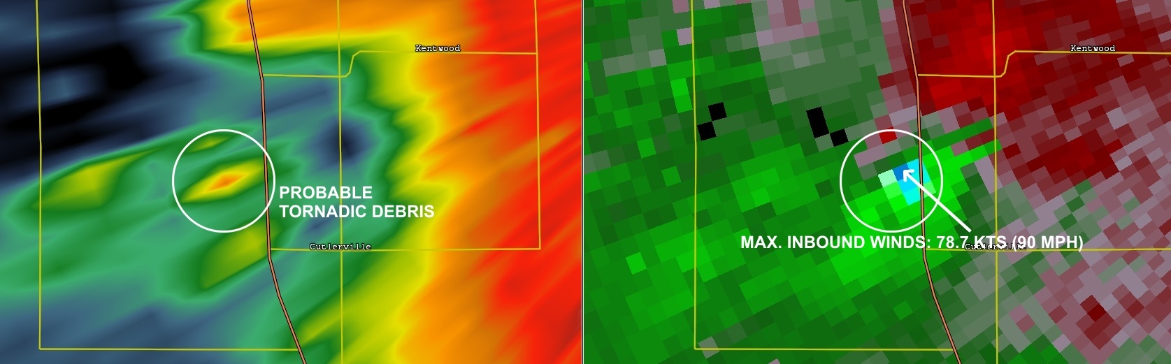
1 scan radar scan later (4 minutes - 10:22 PM EDT), the tornado is just west of US-131 and inbound winds are measured on radar at 78.7 KTS - which is around 90 MPH!  This is 32 MPH MORE than the severe thunderstorm wind threshold.  (Severe thunderstorm winds need to be at least 58MPH for a warning to be called).  Also visible in this radar scan is possible tornadic debris ball, indicated by the area of high reflectivity.

The tornado continues for another 8 minutes or so, continuing to do quite a bit of damage.  During this time, no warnings had been called.  Luckily, no deaths occurred from this storm.

Here is the official tornado track. (Hat tip to the Grand Rapids NWS office for this image).

Why during this entire event were no warnings issued?  Did this just happen to quick for anyone to react?  Looking back at the data, I say no.  Again, I'm writing this article after days of pouring over the data.  I wasn't there as the minutes were ticking.  However, I'm going to go one step further and try to prove that this was no fluke.  I contend that the atmosphere in an around the lower West Michigan at the time of this storm - up to even an HOUR before the tornado was forming - was a loaded gun waiting to happen.

There are a number of key ingredients needed for the formation of a supercell and ultimately a tornado.:  moisture, instability, and wind shear.  It's important to know that not all supercells form tornadoes.  In fact, roughly 20% ever do.  Let's take a look at each of these ingredient factors during the hours leading up to the tornado.

MOISTURE

I'll start with the surface analysis during the time period in question.  This sequence shows that a warm front tracked through the area before the time that the tornado occurred.  The warm front passed overhead around 8PM EDT, but from my estimations, the tornado didn't begin forming until 10PM EDT.  This gave the atmosphere 2 hours to get primed.

 

As a result of the warm front, the dew point, or the measure of how much moisture is present in the air, dramatically increases.  By 10PM EDT, dew points were up to 68 degrees F - which is plenty for the development of severe storms.

INSTABILITY

This next sequence shows MLCAPE (displayed as red contour lines) and MLCIN values (shades of blue) from 3 hours PRIOR to the tornado forming to the time (in my estimation) that the tornado actually formed.

CAPE stands for Convective Available Potential Energy and measures the amount of instability in the atmosphere in Joules (energy) per Kilogram of air.  The "ML" stands for Mean Layer and is an average calculation based on the lowest levels of the atmosphere.   Instability is where a parcel of air is warmer than it's environment, thus is buoyant. Due to this buoyancy, the parcel of air wants to rise further into the atmosphere. This upward movement relates to updraft strength in thunderstorms.  As is illustrated in the sequence above, the amount of CAPE steadily increases to values of 2000 J/kg.  This is certainly enough instability energy to lead to the formation of supercells.  Conversely, CIN (convective inhibition) is steadily DECREASING (goes from blue to white) throughout this same time frame.  CIN can be thought of a force working against CAPE.  Higher CIN values tend to prevent parcels of air from rising.  As CIN is gradually snuffed out air parcels have a better chance of rising.   

WIND SHEAR

Wind shear is a measure (in Knots) of how much winds change direction with height.  Winds at the surface will often be blowing at different directions the higher you move up into the atmosphere.  Supercells become more probable as the effective bulk shear increases through the range of 25-40 kt and greater.

The above sequence shows a persistent shear of at least 30 kts during the time period leading up to and the time of the tornado - well sufficient for tornadoes.

Another measure of shear is called Storm Relative Helicity.  SRH stands for Storm Relative Helicity.  Helicity by itself is the measure of the potential of a fluid (in this case air) to move in a helical (corkscrew) motion.  This is caused by air moving at different speeds and directions in different parts of the atmosphere.  These winds are measured relative the a storm and thus you have Storm Relative Helicity.  By 10PM EDT, SRH values were around 300 M^2/S^2 - which, again, is more than sufficient for the formation of supercells.

 

 

Note that the highest values of 0-3 KM SRM (Storm Relative Helicity) are moving in conjunction with the tornado-forming regions of the storm.

PUTTING THE INGREDIENTS TOGETHER

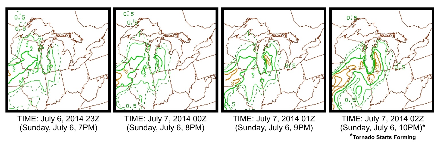
Moving forward, we can use these ingredients to further refine the potential for tornadoes.  CAPE and SRH can be combined together (in a crazy mathematical way that we won't go into here).  From this value get a measurement called EHI or Energy Helicity Index.  This is one of the best measurements for predicting tornadoes.  The following sequence uses the same time frame as the previous examples.

A steady increase in EHI is noted in the time leading up to 10PM.  The value of "4" listed above can actually signify that tornados up to F2 and F3 are possible!

Lastly, using ALL of the measurement ingredients I've discussed so far - Bulk Shear, Storm Relative Helicity, MLCAPE, MLCIN and something called LCL Height (which is a measure of how low clouds are forming in the atmosphere), we can derive something called the Significant Tornado Potential or STP.  According to the SPC, "A majority of significant tornadoes (F2 or greater damage) have been associated with STP values greater than 1, while most non-tornadic supercells have been associated with vales less than 1..."

 

Looking at STP values leading up to the tornado, we see a very small region directly over west Michigan with a value of 2!  In fact, the last sequence shows that area directly over the area hit by the tornado.

 



I hope that I have been able to construct my arguments supporting  the idea that a mini supercell formed in a primed atmosphere and ultimately led to the EF-1 tornado and that this was evident at least one hour prior to the event.  The data is out there - so please feel free to draw your own conclusions.

-Andrew