Altocumulus Castellanus Clouds - The Jellyfish of the Sky

One of the neat things about studying meteorology (and weather in general) is that sometimes you come across something very cool that most people would take for granted.  In my reading about different weather phenomenon a few weeks back, I ran across an article on something called Jellyfish Clouds.  These clouds are fairly rare and form when a layer of moist air rises upwards due to convection and becomes sandwiched between two layers of drier air.  Sometimes when these clouds form, they drop precipitation into the lower dry layer and it begins to evaporate.  The result is a cloud leaving a wispy tail below it which resembles it's namesake - a jellyfish!

On Friday, September 26, 2014, the drive home from work was pretty commonplace and uneventful.  A few miles away from home, I noticed some interesting clouds to my south (yes, I spend a lot of time looking UP at the sky when I probably should be looking at the road!).  Be that as it may, I finished my drive home and when I got into the driveway, I immediately shut off the car and snapped this picture:

 

 I was pretty excited as these looked very much like the jellyfish clouds I had read about a few weeks prior.  However, I didn't want to make too much of it, so I decided to check the sounding data for that day to confirm my suspicions.  I've referred quite a bit to soundings in my previous posts, and it's a topic about which I solely need to devote a topic, but to briefly recap a sounding can be thought of as a cross section of the atmosphere from the ground level all the way up through the troposphere (the area of the atmosphere where all the weather takes place).  Soundings come out at 8AM and 8AM during daylight saving time (7AM and 7PM otherwise).  Data is generated by an instrument called a radiosonde which is attached to a weather balloon.  This instrument and balloon are released from National Weather Service offices all around the country and help meteorologists get an idea of the makeup of the atmosphere above.  They measure temperature, dew point, wind speed and direction.  It was about 6 PM when I arrived home, so the only thing I had at my disposal were the morning sounding.  Here's what it showed:

This graphic contains a TON of information, but the focus for the rest of this article will be on the upper left corner.  This plot - showing the red and green lines - is a graphical depiction of both the temperature (red line) and dew point (green line) starting at the surface (the bottom of the graphic) rising up to some 15-17 km (49,000 - 55,000 ft.) in the air.

 

The first thing you notice is that the red and green lines are fairly close together near the bottom.  The lowest layer - often referred to as the PBL, or Planetary Boundary Layer, shows that due to the proximity of the lines, there is a fair amount of humidity in the air.  Above the PBL, the green line veers sharply to the left.  This indicates that the next layer up is very dry.  Above that, it gets more humid, then dry again, then humid, then dry.  Who knew so much was going on above our heads!!  Here's a better explanation:

 

 

 

In these dry layers, no clouds can form as there is simply not enough moisture.  However, when the lines get close, this indicates that there is sufficient humidity for clouds to form.  In fact, depending on where the layers are, you get different types of clouds!

 

 

 

Remember above when I said that jellyfish (altocumulus) clouds form in a moist layer which is sandwiched between two drier layers?  Well, this is exactly what we had in the atmosphere that day.  In other words, this did confirm to me that, yes, what I had captured earlier were the elusive jellyfish clouds!  From the morning sounding it looks like they were forming above the 6 km (~19,000 ft) mark.  The precipitation which was dropping from them fell into a very dry layer below 6 km.  This was the cause of the wisps beneath the clouds.

 

When the evening soundings were posted, I checked those one last time to see if the data would still support my findings.  Sure enough, although it was quickly drying out, the comparatively humid layer above 6 km was still present.  As I write this article, I'm still jazzed that I was able to capture a fairly rare phenomenon.  Can't wait until the next occurrence!!

 



 

BUT WAIT!  For those of you who haven't dozed off yet, you may have noticed that altocumulus clouds formed in a region where the air temperature is -20 C (-4 F).  How is this possible to have liquid water exist at a temperature below freezing??  Well, believe it or not, this is a process called supercooling and involves a whole branch of could physics (yes, there is such a thing).  This, however, would require it's own article......

 

-Andrew

 

 

 

 

The Dangers of Downbursts from Pulse Severe Thunderstorms

On Saturday, August 16, 2014, the Storm Prediction Center put all of North Texas into it's lowest probability category for severe weather. 

Our area didn't even make it into a SEE TEXT region, yet with our moderately unstable air and weak wind shear environment, conditions were favorable for pulse thunderstorms which were capable of producing a phenomenon called DOWNBURSTS.

A pulse thunderstorm is a single-cell thunderstorm forms and dissipates relatively quickly and typically doesn't yield any severe weather.  However, some pulse storms grow fast enough and drop enough rain to produce a downburst.  A downburst occurs when rain-cooled air falling out of a thunderstorm hits the ground and begins to spread out in all directions.  This expansion of winds (called outflow winds) can sometimes reach 100 MPH and cause quite a bit of damage!  The easiest way to visualize this is to imagine pouring water out of a glass and onto the ground.  As the water slams into the ground, it immediately fans out in all directions, pushing air in front of it.  Is this forward motion that can drive winds as far as 50 miles away from the original storm.  Here is a good visual representation, shown in cross-section. (h/t Wikipedia)

There are actually 2 varieties of downbursts - wet and dry.  A wet downburst happens when rain falling out of the thunderstorm reaches the ground.  A dry downburst happens when rain falling from a storm evaporates before hitting the ground.  In either case, it's the outward-spreading winds from this cooler, sinking air that is responsible for causing damage.  Downbursts smaller than 2.5 miles in diameter are called micro downbursts or microbursts.  Downbursts greater than 2.5 miles in diameter are called macro downbursts or macrobursts.

Let's examine a real-world example of downbursts.  This example begins northwest of Fort Worth, TX.  At 3:02 PM, the National Weather Service issued a severe thunderstorm warning for northwest Tarrant and northeast Parker county.

 

Although the radar returns look unimpressive, there were some interesting things that were about to happen.  One of the dangers with downbursts and the storms associated with them is the speed in which they form, drop their rain-cooled air, and eventually collapse.  The following 5 snapshots of radar reflectivity and radar velocity start at 3:12 PM (about 10 minutes after the initial warning was issued) and ends at 3:31 PM - a span of only 19 minutes!! 

 

TIME 3:12 PM

The first thunderstorm core is in the process of growing. 

 

 

 

TIME 3:17 PM

The first thunderstorm core is still in the process of growing, while a new core is forming to the northwest.

 

TIME 3:22 PM

The first thunderstorm core has matured fully and has begun to produce a downburst (visible on the right side of the image).  The velocity view clearly shows that winds directly underneath the thunderstorm are hitting the ground and are spreading out.  The red colors indicate winds that are blowing away from the radar, while the green colors show winds blowing toward the radar.  The second thunderstorm core continues to grow.

 

 

 

TIME 3:27 PM

The first thunderstorm core is now in the dissipating (or dying) stage.  Reflectivity values (intensity of rain) has dramatically dropped off.  The outflow winds from the original downburst have spread further and further apart.  The second thunderstorm core continues to build up.

 

 

 

TIME 3:31 PM

The first thunderstorm core is now simply an area of heavy rain, while the second thunderstorm core has finally reached its mature stage.  It too has begin to form a downburst beneath itself as indicated by the diverging velocity signatures.

 

 

Let me reiterate that these 2 thunderstorm cores formed, matured, created downbursts, and began to dissipate in about 30 minutes total.  When damage can occur from these storms in such a small amount of time, it's crucial to be aware of the weather in your area.  Boaters and others enjoying open waters are likelier to get caught off guard as the there is little in the way to shield outflow winds that blow across these bodies of water.  Luckily, the downbursts in northwest Tarrant county did not produce any damage to my knowledge.  However, numerous power outages along with downed power lines and trees were reported just north of the downtown Dallas area due so similar conditions.

 

-Andrew

Doppler Radar and Non-Meteorological Targets

One of the cool side benefits of the WSR-88D radars is the ability to detect non-meteorological targets.  Smoke from wild fires, flocks of birds, swarms on insects and even debris from tornadoes can all be seen on radar given the right circumstances.  On Saturday, August 2, 2014, the kids had gotten up extra early, presumably from the excitement of leaving for vacation the next day.  When I sat down at the kitchen table, I noticed that my radar program was still on from the night before.  Gulping down my morning coffee in an attempt to wake up, I noticed something pretty cool.  Here is a time-lapse sequence of what I saw....



See those expanding rings in northeast Dallas and down by Waco?  These are known as Roost Rings.  These rings are actually thousands of birds leaving their nests in their morning hunt for insects.

One way that we can tell that these echoes are biological in nature and not some kind of strange precipitation is by using something called Correlation Coefficient (CC).  This radar product looks at how diverse the radar returns are.  If the values are homogeneous, the higher the CC value will be.  The more values are different, the lower the CC value will be. 

As an example, look at this:

This is a great example of normal precipitation.  The radar beam sees the rain as similar sized drops (more or less) and as a result, the CC values show up with warm colors (reds and oranges). 

Now, look at the roost rings:

The roost rings have very low CC values - which tells us that the objects the radar is seeing are not uniform in size and shape and, more than likely, biological in nature.

Although these roost rings are not uncommon, you usually only see them during the morning hours.  Why is that?  Well, atmospheric conditions play a large role.  During the mornings, there is usually something called a temperature inversion present.  This means that the temperature near the ground is cooler than the air just above it.  As a result, the radar beam gets bent downward (an effect known as superrefraction), making objects near the surface more visible..

Was the July 6th EF-1 Kent County, MI Torndao Caused By a Mini-Supercell?

Today marks the 1-week anniversary of a surprise EF-1 tornado that hit lower West Michigan.  It was a surprise in the sense that apart from an initial severe thunderstorm warning as the system moved over Lake Michigan, no subsequent warnings were issued for the tornado or its parent storm.  I've been pouring over the available data and have come to the conclusion that the tornado shouldn't have been a surprise given the atmospheric conditions of the time.

Let me continue by saying that I'm not a meteorologist and I don't claim to be one.  I am, however, a weather enthusiast who has been studying meteorology for the past number of years.  Hindsight is always 20/20 when it comes to this kind of thing, so what may be perfectly clear now, may not have been as events were unfolding.  Be that as it may, a confirmed EF-1 tornado hit on Sunday night (July 6, 2014) near my hometown of Grand Rapids, MI (well, technically Jenison, MI is my boyhood home town, but it's much easier to say "Grand Rapids).  With all of the advances made over the years in weather forecasting, radar, and public awareness, it seems quite unlikely that something like this could have even happened.  Again, I'm NOT writing to point the finger at anyone.  I really admire the NWS for what they do and look to them as the professionals that they are.  So with that said, what happened? 

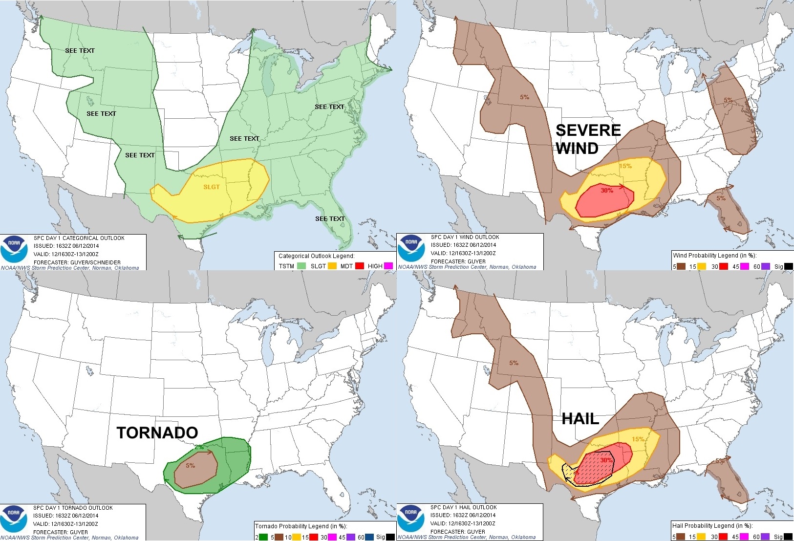
For lower Michigan, Sunday, July 6 was forecast to be in the "general risk" category - having a 5% chance of damaging winds and hail.

By 12:30 PM EDT, the SPC expanded the SLIGHT RISK category eastward.  All of lower Michigan was now forecast to have a 15% chance of damaging winds and hail.

 

The actual text of the outlook reads (emphasis added):

 

THE SLIGHT RISK AREA HAS BEEN EXPANDED NWD/EWD

ACROSS NRN WI INTO UPPER MI AND EWD INTO PARTS OF LOWER MI
CONSISTENT WITH MESOSCALE AND MOST CONVECTION-ALLOWING MODEL
GUIDANCE.  LARGE HAIL AND DAMAGING WING GUSTS ARE EXPECTED TO BE THE
PRIMARY SEVERE HAZARDS BUT AN ISOLATED TORNADO OR TWO MAY ALSO
OCCUR.

 

In other words, based on the forecast weather models and current observations, they raised the possibly of severe weather for the entire region.

 

For the rest of the afternoon, late evening, the weather was non-eventful.  However, around 8:00 PM EDT, storms began forming over Lake Michigan, were intensifying, and racing eastward.   Here is a radar snapshot at 7:58 PM EDT showing moderate to heavy storms north-northwest of Grand Rapids in Oceana, Montcalm and Muskegon Counties.

 

 



As the storms west of Ottawa county came ashore, they intensified to the point that a severe thunderstorm warning was issued.

 

Here is a radar snapshot from 9:04 PM showing 3" hail!

 

 

As a result of the potential damaging hail and damaging winds, the NWS issued the first severe thunderstorm warning 5 minutes later -

 



 

Although this warning originally was set to expire at 10 PM EDT, it was cancelled early - around 9:46 PM - due to the storm falling under severe limits. 

Now here is where things begin to get interesting.  15 minutes later - at 10:01 PM EDT, here is what an un-smoothed radar snapshot looked like:

 

The granular nature of this Level III data easily obscures what I think is the smoking gun.  When the same frame of radar is smoothed.  This is what you get:

 



In my mind, I'm seeing at a very familiar shape - that of a supercell.  However, unlike those supercells that form in the southern plains of the US, this one is smaller - hence a mini-supercell.  (More info on mini-supercells here) Here's an annotated view:

 

Let's compare the above image to an actual supercell which contained a tornado.  Here is a snapshot from the Oklahoma City Radar on May 3, 1999.  The similarities are quite striking.

A close-up of the reflectivity and radial velocity data clearly shows that rotation was beginning to form at 10:01 PM, about 2-3 miles west of the city of Jamestown in Ottawa County.  Red colors show outbound winds (as seen from radar) and green colors indicate inbound winds (as seen from radar).  The red/green juxtaposition clearly indicates cyclonic (counter-clockwise) rotation.

2 scans of the radar - about 8 minutes later (10:09 PM EDT) - a MESOCYCLONE icon shows up.  This is an algorithm built-into the radar that confirms areas of rotation within a storm.  While it's true that these symbols can often be misleading, I contend that this is confirmation that a tornado has already begun to form.  At this time, the area of interest is directly over the Ottawa/Kent county border.

Another 2 scans of the radar go by - about 9 minutes (10:18 PM EDT) and another MESOCYCLONE icon shows up.  This time it indicates that the rotation is not as deep.  The placement seems a bit off too.  This could be a function of the imprecise algorithm.  However, the center of rotation (as derived from velocity data) is consistent with the NWS's claim that the tornado formed about 10:20 PM EDT roughly 4 miles west of Cutlerville.

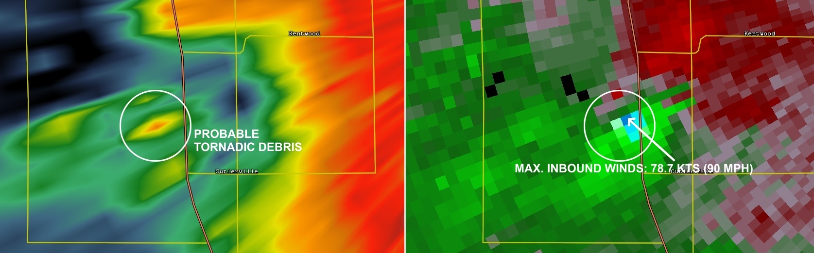
1 scan radar scan later (4 minutes - 10:22 PM EDT), the tornado is just west of US-131 and inbound winds are measured on radar at 78.7 KTS - which is around 90 MPH!  This is 32 MPH MORE than the severe thunderstorm wind threshold.  (Severe thunderstorm winds need to be at least 58MPH for a warning to be called).  Also visible in this radar scan is possible tornadic debris ball, indicated by the area of high reflectivity.

The tornado continues for another 8 minutes or so, continuing to do quite a bit of damage.  During this time, no warnings had been called.  Luckily, no deaths occurred from this storm.

Here is the official tornado track. (Hat tip to the Grand Rapids NWS office for this image).

Why during this entire event were no warnings issued?  Did this just happen to quick for anyone to react?  Looking back at the data, I say no.  Again, I'm writing this article after days of pouring over the data.  I wasn't there as the minutes were ticking.  However, I'm going to go one step further and try to prove that this was no fluke.  I contend that the atmosphere in an around the lower West Michigan at the time of this storm - up to even an HOUR before the tornado was forming - was a loaded gun waiting to happen.

There are a number of key ingredients needed for the formation of a supercell and ultimately a tornado.:  moisture, instability, and wind shear.  It's important to know that not all supercells form tornadoes.  In fact, roughly 20% ever do.  Let's take a look at each of these ingredient factors during the hours leading up to the tornado.

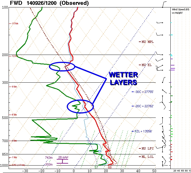
MOISTURE

I'll start with the surface analysis during the time period in question.  This sequence shows that a warm front tracked through the area before the time that the tornado occurred.  The warm front passed overhead around 8PM EDT, but from my estimations, the tornado didn't begin forming until 10PM EDT.  This gave the atmosphere 2 hours to get primed.

 

As a result of the warm front, the dew point, or the measure of how much moisture is present in the air, dramatically increases.  By 10PM EDT, dew points were up to 68 degrees F - which is plenty for the development of severe storms.

INSTABILITY

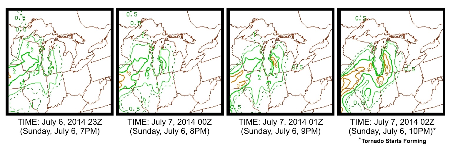
This next sequence shows MLCAPE (displayed as red contour lines) and MLCIN values (shades of blue) from 3 hours PRIOR to the tornado forming to the time (in my estimation) that the tornado actually formed.

CAPE stands for Convective Available Potential Energy and measures the amount of instability in the atmosphere in Joules (energy) per Kilogram of air.  The "ML" stands for Mean Layer and is an average calculation based on the lowest levels of the atmosphere.   Instability is where a parcel of air is warmer than it's environment, thus is buoyant. Due to this buoyancy, the parcel of air wants to rise further into the atmosphere. This upward movement relates to updraft strength in thunderstorms.  As is illustrated in the sequence above, the amount of CAPE steadily increases to values of 2000 J/kg.  This is certainly enough instability energy to lead to the formation of supercells.  Conversely, CIN (convective inhibition) is steadily DECREASING (goes from blue to white) throughout this same time frame.  CIN can be thought of a force working against CAPE.  Higher CIN values tend to prevent parcels of air from rising.  As CIN is gradually snuffed out air parcels have a better chance of rising.   

WIND SHEAR

Wind shear is a measure (in Knots) of how much winds change direction with height.  Winds at the surface will often be blowing at different directions the higher you move up into the atmosphere.  Supercells become more probable as the effective bulk shear increases through the range of 25-40 kt and greater.

The above sequence shows a persistent shear of at least 30 kts during the time period leading up to and the time of the tornado - well sufficient for tornadoes.

Another measure of shear is called Storm Relative Helicity.  SRH stands for Storm Relative Helicity.  Helicity by itself is the measure of the potential of a fluid (in this case air) to move in a helical (corkscrew) motion.  This is caused by air moving at different speeds and directions in different parts of the atmosphere.  These winds are measured relative the a storm and thus you have Storm Relative Helicity.  By 10PM EDT, SRH values were around 300 M^2/S^2 - which, again, is more than sufficient for the formation of supercells.

 

 

Note that the highest values of 0-3 KM SRM (Storm Relative Helicity) are moving in conjunction with the tornado-forming regions of the storm.

PUTTING THE INGREDIENTS TOGETHER

Moving forward, we can use these ingredients to further refine the potential for tornadoes.  CAPE and SRH can be combined together (in a crazy mathematical way that we won't go into here).  From this value get a measurement called EHI or Energy Helicity Index.  This is one of the best measurements for predicting tornadoes.  The following sequence uses the same time frame as the previous examples.

A steady increase in EHI is noted in the time leading up to 10PM.  The value of "4" listed above can actually signify that tornados up to F2 and F3 are possible!

Lastly, using ALL of the measurement ingredients I've discussed so far - Bulk Shear, Storm Relative Helicity, MLCAPE, MLCIN and something called LCL Height (which is a measure of how low clouds are forming in the atmosphere), we can derive something called the Significant Tornado Potential or STP.  According to the SPC, "A majority of significant tornadoes (F2 or greater damage) have been associated with STP values greater than 1, while most non-tornadic supercells have been associated with vales less than 1..."

 

Looking at STP values leading up to the tornado, we see a very small region directly over west Michigan with a value of 2!  In fact, the last sequence shows that area directly over the area hit by the tornado.

 



I hope that I have been able to construct my arguments supporting  the idea that a mini supercell formed in a primed atmosphere and ultimately led to the EF-1 tornado and that this was evident at least one hour prior to the event.  The data is out there - so please feel free to draw your own conclusions.

-Andrew

Severe Weather Likely For North Texas Today

Today, the SPC (Storm Prediction Center) has put North Texas in the SLIGHT RISK area for severe weather.

The main threats today will be for large hail (up to baseball size!) and damaging winds.  However, an isolated tornado threat cannot be ruled out.

What's causing all of this today?  First, let's take a look at the atmosphere.

This chart, referred to as a SKEW-T diagram, is generated from an instrument called a Radiosonde.  This instrument is attached to a balloon.  Twice a day, local weather service offices release these balloons so meteorologists can get an idea of the atmosphere.  The red solid line is a plot of temperature from the surface (at the bottom of the chart) all the way up into the atmosphere.  The top of this chart is over 15 km high!  The solid green line is the plot of the dewpoint, or the amount of moisture in the atmosphere.

If you follow the temperature plot from the surface, you see that it goes to the right.  Then, higher up, it turns back to the left.  When the temperature plot moves right as you go up, this is called a temperature inversion.  In other words, the air is getting WARMER as you go higher, no colder as you would expect.  This temperature inversion, called the CAP, limits storm potential. 

But just above the CAP, the temperature curve heads left FAST.  In other words, the temperature gets very cold, very fast.  This creates a condition called INSTABILITY.  Think of it this way:  if a ball (or parcel) of warm air at the surface can get lifted up past the cap, the warm air will begin to rise on its own - because it's warmer than the air surrounding it.  The warmer the air, the faster it will rise, the faster it rises, the higher in the atmosphere it gets.  This, among other factors, is what leads to a large hail risk. 

An important thing to note is that because of a CAP, air doesn't just rise up on it's own and become buoyant (well, it can sometimes - but that's for another topic).  In order for it to get above the CAP, it has to have help.  Typically some sort of lifting mechanism is needing to help the air rise.  In today's forecast, we're expected to have a cold front surge south.  When this colder air (which is heavier than warm air) comes into the area, it helps to lift the warmer, moister air that's already present up past the CAP.  This is why storms typically form in front and along cold fronts.

Another similar lifting mechanism is an outflow boundary.  This is a wave of cool air that gets pushed out and away from other thunderstorms. The storms earlier this morning (some of which became severe) formed along an outflow boundary which was created from decaying thunderstorms in Oklahoma overnight.

The image above shows the approximate location of the outflow boundary this morning.  It's represented by the black dotted/solid line.  This provided the lift needed for this morning's storms.

Our local National Weather Service office recently issued this graphic.

While the DFW Metroplex is still in a severe risk area, the greatest risk for today will be around and south of the previously discussed outflow boundary. 

Stay safe today and keep an eye to the skies!

-Andrew

Doppler Radar -So Many Colors, So Much Information

One of the things that really got me interested in weather was Doppler Radar.  I was fascinated with how radar could tell meteorologists about what was happening outside - simply by looking at colors on a screen.  Of course radar isn't the only tool in the meteorologist toolkit, but it is one of the strongest and most important.  The current generation of radar used today by the National Weather Service (NWS) is the WSR-88D.  This stands for Weather Surveillance Radar - 1988 Doppler.  The NWS (and other agencies including NOAA and the Department of Defense) operate some 164 radar sites throughout the continental US, Hawaii, Alaska, Puerto Rico and Guam.

Doppler radar works on a very simple principal - "speaking" and "listening".  In essence, the radar "speaks" by sending out pulses of electro-magnetic energy (microwaves) to some target.  Most of that energy is scattered, but a small portion is reflected back to the radar site where it is "heard".  The amount of returned data (e.g. how loud the echo is) is called "reflectivity" and is measured in units of decibels of Z or dBZ.    This VERY basic example is done thousands of times per second at the speed of light.  In fact, a WSR-88D radar is "speaking" for just about 7 seconds per hour and the remaining 59 minutes, 53 seconds is spent "listening" for any returned signals.  Because we know the speed at which these signals are sent (the speed of light) and the time it takes for the signals to return (and something else called a Phase Shift) we can also determine if an object is stationary or moving towards or away from the radar and the speed its moving .  Isn't math AWESOME?? 

Let's take a look at what reflectivity and velocity look like in real-world examples.  Here is a screen shot of a supercell thunderstorm approaching Oklahoma City on May 7, 2014.  The left pane is showing reflectivity - or the intensity of the echoes being returned to the radar.  The right pane is radial velocity - showing winds blowing toward the radar (GREEN) or away from the radar (RED).  While these two different views are looking at the same space and time, the information they show is vastly different. The full resolution image can be found here.

Let's zoom in on reflectivity...(full resolution)

 

In reflectivity mode the color scale is completely arbitrary, but it's generally agreed upon that warmer colors indicate higher reflectivity and cooler colors indicate areas of lower reflectivity.  Using that model, we can see that cities like Spencer, OK and Mustang, OK are getting this heaviest precipitation, while cities like Piedmont, OK and Bridge Creek, OK are getting very little precipitation.

 

 

In velocity mode, keeping in mind that green indicates winds blowing toward the radar and red indicates winds that are blowing away from the radar, we can clearly see that the area by Bridge Creek has winds blowing "inbound" and by Tuttle, the windows are blowing "outbound".  This is actually an area of broad circulation that should be watched as it could potentially tighten in turn into a tornado.

 

Here's a close up of that area with the wind directions annotated.  With the arrows present, the rotation becomes much more apparent.

 

 

Reflectivity and Velocity products are very adept at telling meteorologists what is happening - however, they're lacking in some critical information.  However, in 2013, a major upgrade to the network of WSR-88D's was completed.  This "Dual-Pol" upgrade (short for Dual Polarization) gave meteorologists a number of new tools to help identify more accurately what the radar is "seeing".  Before the upgrade, the beam that the radar was sending out was only polarized in one direction (let's say horizontal).  Therefore, the radar could only measure the width something it hit, not the height.  Thus, critical information about the type of precipitation was lacking.  Think of it this way:  When a rain drop is falling, it's not perfectly spherical.  Because of the effects of air resistance, a rain drop will actually become oblate.  I like to think of this as a hamburger bun shape.  The bigger the rain drop, the flatter (or wider) it becomes as it falls.  Let's then contrast this with a hail stone of the same width.  Even though both objects may be similar in width, they are not the same in height.  The rain drop has a much narrower dimension vertically.  A hail stone (a sphere in this basic example), has roughly the same dimensions vertically and horizontally when falling.  Therefore, a single-polarized radar beam had trouble distinguishing between rain and hail.

Enter DUAL-POL.  Like I stated before, this stands for Dual-Polarization.  This means that the radar can "see" in both the horizontal AND vertical dimensions.  Using the example above, a large rain drop will be wider than it is taller when falling.  Hail will be roughly spherical in shape when it falls.  Therefore, the difference between the vertical and horizontal measurements of  the target can now be better distinguished and more easily identified.  This "differential reflectivity" is a major benefit to the dual-polarization upgrade as meteorologists can get a better idea if an area of a storm contains heavy rain as opposed to hail.  This new set of information can better assist meteorologists in the warning decision process by refining areas of more severe weather.

One other important benefit of this dual-polarization upgrade is the ability to determine how similar targets are in size and shape.  For example, if in a given scan, all of the targets are roughly the same size and same shape, one can infer that the precipitation is homogeneous.  Areas of rain only, can now be distinguished from areas of rain AND hail mix.  This product is called "Correlation Coefficient".  There are other, more technical, products that the dual-polarization upgrade offers, but for this article, I'll leave them out. 

So, big deal, right?  What's all the fuss?  Let me wrap it all up by showing one last example.  The screen shot below was taken on April 28, 2014 from the KGWX Doppler Radar near Columbus Air Force Base in Mississippi.  The full resolution image is here.



This 4-pane view is looking at the same area in both space and time, but is displaying vastly different data.  The upper left corner, is radar reflectivity.  The upper right is radial velocity.  The lower right is something called storm-relative radial velocity.  This is similar to radial velocity, but it displays the speeds of the winds with the motion of the storms subtracted.  This helps to identify movement of winds within a storm without having the storm motion factored in.  Lastly, the lower left pane is the correlation coefficient product - one of the new dual-pol upgrade products.

Reflectivity

One key feature that this image of radar reflectivity shows is a distinct "hook echo" shape.  I've annotated this in the following image.  See how the rain wraps around in the shape of a hook?  While this hook shape is certainly interesting, on its own, it can't give us the full picture of what's really going on.

Velocity

The velocity view, again, shows winds that are blowing toward (GREEN) and away (RED) from the radar.  In this example the radar site is located well BELOW the image.  This is important to know as inbound and outbound winds are measured relative to the radar site.   See how in both images, you have reds and greens very close together?  This is a very good indicator that there is very strong rotation present.  The closer and brighter the colors are together, the stronger and tighter the winds are.  Here's an annotated view:

Up to now, we have a pretty good indication that there is something major going on.  However, we cant be 100% certain as we're not present to witness the actual event.  Let's add the last component to see if we can get a full picture.

Correlation Coefficient

 

Again, this product looks at how similar in size and shape the precipitation is.  For the most part, the reds and purples tell us that, yes, what we see from the reflectivity view shown earlier is just rain.  The yellows and oranges shown near the top are probably hail.  However, the main focus of this image is that large, gaping hole in the middle.  See that blue section?  This is where "similarness" of what the radar is seeing drops down dramatically.  If you were to superimpose this image directly over that of the velocity data, the areas where the winds are coming together and this blue area are exactly lined up.  In this example what we're seeing is a tornadic debris ball.  This is "stuff" that a tornado is picking up and lofting into the air.  It could be houses, it could be vehicles, it could be trees, bushes or farm animals.  Regardless, this tornado was not just radar indicated, but verified by storm spotters.  This debris ball signature could not be possible with out the recent dual-pol upgrade.

 

The dual-polarization upgrades not only were time-intensive, but they were also costly - about $50 million dollars in all.  However, the wealth of new information that this technology has given and the better ability of meteorologists to improve the warning process, in my view, justifies the cost.  While meteorologists never rely on radar data alone in the warning decision process, important upgrades like dual-pol help to verify and substantiate reports from the public and most importantly save lives.

-Andrew